Delivering daily insights in DS, ML, RAGs, Agents & AI Engineering. Trusted by over 100k+ readers!
Join for free →
Joined May 2022
- Tweets2.9K
- Following2
- Followers51.9K
- Likes2.6K




Pinned Tweet
Get a FREE Data Science E-book (530+ page), featuring over 150 essential lessons in data science and machine learning.
Download link in profile.
Daily Dose of Data Science retweeted

Big win for AI Engineers!
If you're deploying agents in production, this one is for you.
(bookmark it)
There's a new system that can test and evaluate your agents against the real world, then write the fixes, all before you deploy them.
AI agents look great in demos, until real users start breaking them. Your agent can tell a customer "refund done" on a $1,080 invoice without ever checking who she is, and the logs will still look clean.
Normally you only find a failure like that after a real customer runs into it. @pluraiAI Simulation lets your agent fail in a simulated world first, so you can fix the problem before any user sees it.
↳ It rebuilds your actual agent, its tools and its environment from your code
↳ Simulated users push the agent into the edge cases that matter for your use case
↳ Evals built for your agent check the actions it took, like whether it verified the customer before issuing that refund
↳ Every failure comes with the run that exposed it and a fix you can verify
↳ Any production failure can become a simulation you replay against every new version
It ships as a single plugin for coding agents like Claude Code and Codex, and it works with whatever agent you're building. I've started running it on my own agents too.
It's free for every AI engineer. Link in the first comment.
I worked with the Plurai team to put this together. Here's the whole system, step by step, from the first simulated user to a re-tested fix:
MCP meets agent skills.
MCP already gave agents a standard way to connect to tools, resources, and external systems.
Now it also defines a standard way to discover and load Agent Skills directly from MCP servers.
The flow is simple:
→ Connect to an MCP server
→ Discover available skills
→ Inspect skill metadata
→ Load the relevant SKILL.md only when needed
Under the hood, Skills are served through MCP’s existing Resources primitive.
That means SKILL.md, references, scripts, examples, and other supporting files are exposed as resources that the client can read on demand.
This is especially useful for context-window management.
Instead of loading every workflow instruction upfront, the agent can first discover what skills are available and pull in only the one required for the current task.
A useful mental model is:
Tools = what the agent can do
Resources = what the agent can access
Skills = how the agent should perform a reusable workflow
Previously, that workflow knowledge often lived separately in docs, repos, prompt files, or custom integrations.
Now the MCP server can expose the capability and the playbook for using it together.
So we get:
→ Standardized skill discovery
→ On-demand context loading
→ Cleaner distribution and versioning
→ Reusable workflows that travel with the server
MCP was already the connection layer.
Skills now add a standardized way to ship reusable agent know-how on top of it.

ALT Diagram showing how MCP servers expose Agent Skills and their supporting files as on-demand resources.
Daily Dose of Data Science retweeted

72 techniques to optimize LLMs in production:
(bookmark this)
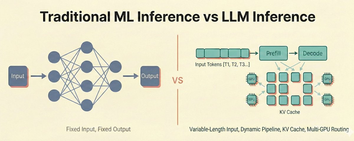
LLMs break every assumption about regular ML inference.
A traditional ML model (CNN, transformer classifier, XGBoost) produces its output in a single forward pass.
Nothing carries over between requests. The GPU does the same kind of work each time.
LLMs don't work like that.
The output is generated one token at a time, autoregressively, which turns a single request into hundreds of sequential forward passes.
The prefill stage is compute-bound, while decode is memory-bandwidth-bound, and running them together on the same GPU hurts both.
The KV cache grows with conversation length and is shared across requests, so routing is no longer about least-busy servers but about which replica already has the relevant prefix cached.
MoE models add expert parallelism on top of that.
None of this exists in traditional ML serving.
That is why an entirely new stack of optimizations has emerged specifically for LLM inference, spanning compression, attention, KV cache management, batching, decoding, parallelism, and routing.
I recently mapped out 72 techniques that optimize LLMs in production, grouped into nine pillars.
I recently wrote an article (shared below) that covers how LLM inference differs from regular ML inference and why each of these pillars exists.
Over to you: What other LLM optimization techniques would you add here?

Daily Dose of Data Science retweeted
RAG vs. Graph RAG vs. Agentic RAG, clearly explained!
Standard RAG embeds documents into vectors and retrieves the most similar chunks via similarity search. For direct factual lookups, this works well.
But it breaks down when a query needs to connect facts spread across multiple documents. Similarity search retrieves individual chunks, not the relationships between them.
Graph RAG adds a knowledge graph layer on top.
→ During indexing, an LLM extracts entities and relationships from the documents.
→ During retrieval, the system traverses these connections instead of relying on embedding similarity alone.
This is what enables multi-hop queries.
Say a vector DB stores three facts about internal services:
↳ "The checkout service uses payments API."
↳ "The payments API runs on cluster-3."
↳ "Cluster-3 is scheduled for maintenance on Friday."
Someone asks: "Will the checkout service be affected by Friday's maintenance?"
Vector search can likely retrieve facts 1 and 3 because the query mentions "checkout service" and "Friday maintenance."
But it will miss fact 2, which connects the payments API to cluster-3.
That middle fact sits too far from the query in embedding space. It mentions neither "checkout" nor "maintenance," so it never makes it into the retrieved context.
A knowledge graph connects these as linked entities, and graph traversal finds the full path in one query.
Agentic RAG takes a different approach entirely.
Instead of a fixed retrieval pipeline, an LLM agent decides at query time which tools to invoke, which sources to query, and in what order.
Check the visual below to understand the three architectures thoroughly.
One thing to note here is that these three aren't levels of sophistication that you need to graduate through.
Instead, they solve different query types.
↳ Single-hop factual lookups → standard RAG
↳ Multi-hop relationship queries → Graph RAG
↳ Dynamic multi-source tasks with tool use → Agentic RAG
Once the right architecture is in place, the next leverage point is efficiency.
Most RAG architectures rely heavily on vector search, and that layer can be made 32x more memory-efficient using binary quantization.
I covered the full implementation in the article below.
👉 Over to you: Which RAG architecture are you running in production?

Insane progress for small language models!
MiniCPM5-2B is a dense 2B-parameter model by OpenBMB from China that is built for reasoning, coding, and tool use on resource-constrained hardware.
The model specifically excels at coding and tool calling, two capabilities central to the shift from on-device LLMs to on-device agents.
Instead of only answering prompts, it can use tools, generate code, carry information between steps, and complete multi-step tasks.
We ran it 100% locally and connected it to a small investigation agent with one request:
> Revenue dropped last week. Investigate what happened, quantify the impact, identify the likely cause, and produce an incident report with supporting evidence.
The evidence was spread across orders, traffic, payments, refunds, and deployment logs.
The model inspected the files, wrote its own queries, analyzed the intermediate results, and decided what to investigate next.
Each tool result informed the next action, so the final report depended on the model maintaining a coherent investigation across the complete trajectory.
The recording shows the actual task from beginning to end. It starts with the revenue question, follows the tool calls and supporting evidence, and ends with a quantified diagnosis and incident report.
The data, tool execution, and model inference all remained on our machine.
These capabilities were optimized through Agentic Pre-training, SFT, and large-scale RL. They do not come entirely from an application-level agent framework.
MiniCPM5-2B supports SGLang, vLLM, llama.cpp, Ollama, iOS, Android, and HarmonyOS.
OpenBMB has also released the model weights and parts of the training recipes and data resources behind it.
A 2B model can now maintain enough state to coordinate tools and complete a useful investigation on local hardware.
Daily Dose of Data Science retweeted
NVIDIA released a new RL framework:
Your entire setup is one Python file:
- write a class with a step() function
- return a reward from it
- the framework handles the rest, up to 1T-class MoE training
In a typical RL framework, the environment and reward logic are added inside the trainer's codebase.
Adding a new task requires writing framework code, registering it, and wiring up config for it.
The reward usually comes from a separately trained reward model, which needs its own GPUs and placement next to the actor and critic.
NVIDIA's Molt framework drops both these requirements.
Every run takes an agent_path flag pointing to one Python module, and the trainer code never changes.
The module gives you two ways to plug in an agent.
> The first is an Env class where you write a step() function that receives the model's output and returns a reward, and the framework handles everything else, i.e., calling the model, tokenizing, and looping turn after turn until the episode ends.
> The second is a ChatAgent class, for agents that already exist as their own loop. Here, you write the loop yourself, calling the model through a standard OpenAI or Anthropic client, and the framework spins up a local server so those calls hit its vLLM engines instead of an external API.
Either way, the trainer sees the same thing, i.e., a trajectory of tokens and a reward at the end.
That reward can come from a string-match grader, code executed in a sandboxed subprocess, or an LLM-as-judge call.
So there is no reward model to train or place, and no environment code living inside the framework.
Under the hood, Molt runs a single trainable actor (plus an optional critic for PPO) on FSDP2, vLLM engines for rollout, and Ray queues between them, so generation, training, and weight sync overlap instead of running in lockstep.
Scaling just requires setting some flags on the same command.
The framework also splits the model across GPUs for you, so the script that trains an 8B model on one node can also train DeepSeek-V3-scale MoE models on a cluster by raising the parallelism flags.
Here's the repo: github.com/NVIDIA-NeMo/labs-…
Since the framework is new, I am still experimenting with it and will share more about my learnings soon.
To dive deeper into how top AI labs are building RL Agents in 2026, I wrote a full article about it.
It covers the evolution from RLHF to GRPO with verifiable rewards and using an LLM-as-judge reward function. This idea extends RL training to non-verifiable agentic tasks without writing custom reward functions.
Read it below.

CPU vs GPU vs TPU vs NPU vs LPU, explained visually:
(bookmark this)
5 hardware architectures power AI today.
Each one makes a fundamentally different tradeoff between flexibility, parallelism, and memory access.
> CPU
It is built for general-purpose computing. A few powerful cores handle complex logic, branching, and system-level tasks.
It has deep cache hierarchies and off-chip main memory (DRAM). It's great for operating systems, databases, and decision-heavy code, but not that great for repetitive math like matrix multiplications.
> GPU
Instead of a few powerful cores, GPUs spread work across thousands of smaller cores that all execute the same instruction on different data.
This is why GPUs dominate AI training. The parallelism maps directly to the kind of math neural networks need.
> TPU
They go one step further with specialization.
The core compute unit is a grid of multiply-accumulate (MAC) units where data flows through in a wave pattern.
Weights enter from one side, activations from the other, and partial results propagate without going back to memory each time.
The entire execution is compiler-controlled, not hardware-scheduled. Google designed TPUs specifically for neural network workloads.
> NPU
This is an edge-optimized variant.
The architecture is built around a Neural Compute Engine packed with MAC arrays and on-chip SRAM, but instead of high-bandwidth memory (HBM), NPUs use low-power system memory.
The design goal is to run inference at single-digit watt power budgets, like smartphones, wearables, and IoT devices.
Apple Neural Engine and Intel's NPU follow this pattern.
> LPU (Language Processing Unit)
This is the newest entrant, by Groq.
The architecture removes off-chip memory from the critical path entirely. All weight storage lives in on-chip SRAM.
Execution is fully deterministic and compiler-scheduled, which means zero cache misses and zero runtime scheduling overhead.
The tradeoff is that it provides limited memory per chip, which means you need hundreds of chips linked together to serve a single large model. But the latency advantage is real.
AI compute has evolved from general-purpose flexibility (CPU) to extreme specialization (LPU). Each step trades some level of generality for efficiency.
The visual below maps the internal architecture of all five side by side.
To dive deeper into GPUs specifically, we also wrote a detailed article on how they work.
It builds up from first principles why memory and compute compete, why that gap exists in the hardware, and what makes a workload memory-bound in the first place.
Read it below.


Stateful vs. Stateless MCP core.
(Anthropic's biggest MCP update)
Let us explain what that means:
Until this release, talking to an MCP server worked like a phone call. Both sides ran an initialize handshake, and the server returned a session id carried on every later request.
That session was a live object inside one specific server process, holding the negotiated state.
Picture a restaurant where the waiter who took the order is the only one who knows what was ordered. Everything works until that waiter goes home.
Because that state lives in one process, a balancer could not spread requests across three MCP server instances. Teams pinned clients with sticky sessions or pushed session state into shared storage, which blocked autoscaling and made a single restart drop every open session.
The latest update deletes all of it. The handshake and the Mcp-Session-Id header are gone, and each request now carries its own protocol version, client identity, and capabilities in a _meta field.
Clients that want the capability list up front can call server/discover, but nothing requires it.
The restaurant works the other way around now. That flips the restaurant around. Every request is a written order slip now, and any waiter can fill it.
So any request can land on any instance behind a plain round-robin balancer, with no shared session store. MCP servers become ordinary HTTP services that run on serverless and edge, and survive restarts.
Removing sessions broke three features, so each got rebuilt.
→ Tools that need to ask the user something mid-call used to push that request down a held-open stream. Now the server returns input_required and the client retries with the answers attached.
→ Method and tool names moved into the Mcp-Method and Mcp-Name headers, so a gateway or rate limiter can route and meter without parsing the JSON-RPC body.
→ List responses carry ttlMs and cacheScope, so clients cache tool catalogs instead of refetching them on every reconnect.
State did not disappear here, it moved somewhere the model can see it.
Applications that need continuity get an explicit handle from a tool and have the model pass it back as an argument on the next call.
A session id in a header is invisible to the model, while a handle in the arguments is something it can read, thread between tools, and recover from after a failed call.
Since we are on MCP, we also wrote about why the MCP versus CLI debate was the wrong one, and how agents can call tools by writing code instead of loading every schema into context.
The article is quoted below.

Daily Dose of Data Science retweeted
Chat with video using EmbeddingGemma 2 (100% local):
EmbeddingGemma 2 by @GoogleDeepMind maps text, images, video, and audio into a shared vector space. This makes it possible to search video frames with natural language.
Devs have already built native Rust implementations for local inference.
Unsloth also provides a 176 MB, 4-bit GGUF checkpoint for text embeddings, although that version doesn't include the full multimodal pipeline.
I tested the video-search use case by building a chat interface that finds matching frames and jumps to their timestamps.
On my Apple M3 Pro, using the CPU:
- Indexing took 29s for a 60s video
- Search took 25 ms on average across 9 queries
- The saved frame vectors occupied 180 KiB.
The video is indexed once. Each new search embeds the query and compares it with the saved frame vectors. Processing stays entirely on the laptop.
The video below depicts the entire flow in action.
That said, model quantization reduces the memory needed for the weights. The retrieval index has its own storage cost, which grows as you add videos.
To dive deeper into reducing that cost, I wrote a full article on binary quantization.
It explains how storing vectors with one bit per dimension reduces their raw storage by 32x compared with float32, and includes a working retrieval implementation.
Read it below.
Daily Dose of Data Science retweeted
8 AI model architectures, visually explained:
LLMs get so much attention that it's easy to overlook the rest of the field. Different inputs, tasks, and deployment constraints have led to very different model designs.
Here are eight specialized AI model architectures:
1. LLM (Large language models)
Text is split into tokens, mapped to embeddings, and processed through transformer layers. The model generates its response by predicting successive tokens.
↳ GPT, Claude, Gemini, Llama.
2. LCM (Large concept models)
Moves prediction to the sentence level. Sentences become SONAR embeddings, and the model predicts the next sentence representation. Meta explored both autoregressive and diffusion-based versions.
↳ Meta's LCM research introduced this approach.
3. LAM (Large action models)
Connects a user's request to actions in an environment. These systems interpret intent, plan steps, and use interfaces or tools, often checking results before continuing.
↳ Rabbit R1, Microsoft UFO, Claude Computer Use.
4. MoE (Mixture of experts)
A router assigns token representations to selected expert networks inside the model. Activating a subset of experts adds model capacity without running every expert for every token.
↳ Mixtral, DeepSeek, Switch Transformer.
5. VLM (Vision-language models)
Combines visual representations with language processing. A vision encoder extracts image features, which are connected to a language model so it can answer questions about visual content.
↳ GPT-4V, Gemini, LLaVA.
6. SLM (Small language models)
Uses fewer parameters to reduce memory and compute requirements. These models can run locally, with quantization often reducing their deployment footprint further.
↳ Phi-3, Gemma, Mistral 7B, Llama 3.2 1B.
7. MLM (Masked language models)
Learns by predicting hidden tokens using context on both sides. This bidirectional training produces representations useful for retrieval, classification, and other language-understanding tasks.
↳ BERT, RoBERTa, DeBERTa.
8. SAM (Segment Anything Model)
An image encoder processes the image, while a prompt encoder handles points, boxes, or masks. A mask decoder combines them to identify the requested regions.
↳ Meta's SAM supports interactive segmentation and image annotation.
These aren't eight mutually exclusive categories. A small model can process images, and a language model can use MoE layers. Some labels describe architecture, while others describe training or intended use.
There's another approach I kept outside the image because it alters how a model handles context rather than introducing a separate model family.
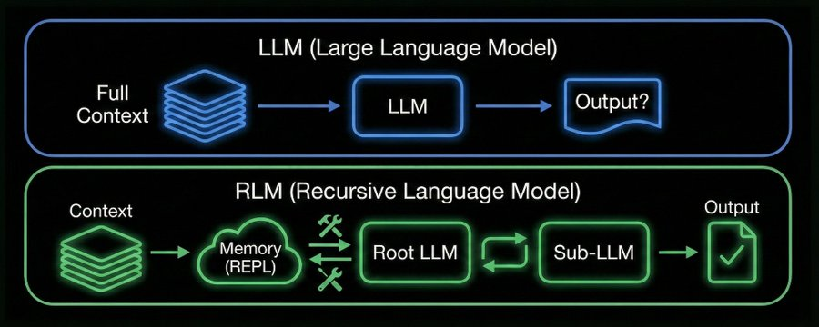
Recursive language models, from MIT, put the input into a Python environment that a root model can inspect through code.
The model can search or slice that input, then make recursive model calls on selected portions instead of loading everything into its own context window.
The reported experiments handled inputs beyond 10 million tokens without retraining, with gains over the base model even on some tasks whose inputs already fit its context window.
I recently wrote a full breakdown of how this works, including why accessing a large input and reasoning reliably over it are different problems.
Read it below.
A good technical LLM interview question:
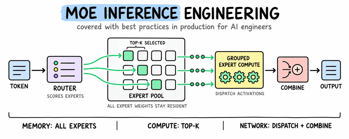
We replace a dense feed-forward layer with a top-2 MoE.
The profiler confirms that the MoE executes fewer FLOPs per token.
However, end-to-end inference latency has increased instead of decreasing.
Why did this happen?
A standard Transformer applies the same feed-forward network to every token in a layer.
An MoE layer replaces that network with multiple experts. Each expert is a feed-forward network with its own weights.
A router reads each token’s hidden-state vector, scores the available experts, and selects the top two. It also produces a routing weight for each selection.
Only those selected experts process the token. The model therefore contains many expert weights while executing only a small subset for each token.
The serving system must move activations when the selected experts are stored on different GPUs.
The visual follows a batch that begins on GPU 0.
The router returns two expert IDs and two routing weights per token. One selected path is shown for each example token to keep the diagram readable.
Token T1 selects E1 on GPU 0. Its activation remains in local GPU memory, where E1 processes it.
T2 selects E4 on GPU 1 in the same server. GPU 0 transfers the activation through NVLink, a high-bandwidth GPU-to-GPU connection. NVSwitch connects several GPUs through this fabric.
T3 selects E7 on GPU 2 in another server. Its activation crosses the cluster network through InfiniBand or Ethernet.
To be clear, the system transfers activation vectors, which are the numerical representations produced for a token by the preceding Transformer operations.
Each destination GPU runs its expert and returns the output to GPU 0.
GPU 0 multiplies both selected expert outputs by their routing weights, adds them together, and restores the original token order.
Different tokens can select different expert pairs. Across a batch, those assignments may involve every GPU storing experts.
Each GPU may therefore send activations to several GPUs while receiving activations for its own experts. This exchange is called all-to-all communication.
And there are several ways to optimize this.
For instance, keeping frequently selected experts within the same server reduces remote traffic.
Balanced routing prevents one GPU from delaying the layer.
Communication overlap allows local expert computation to continue while remote activations move.
In this setup, sparse routing reduces expert FLOPs, but token dispatch and network communication erase part of that saving.
If you want to dive deeper, we recently covered MoE inference engineering, including routing, expert placement, token dispatch, load balancing, communication overlap, memory, quantization, and offloading.
Read the article below.
Daily Dose of Data Science retweeted
7 MoE routing strategies in production, clearly explained:
(bookmark this)
Sending every token to its highest-scoring experts can make an MoE model slower.
The problem is that many tokens can prefer the same experts. Those experts become overloaded while others remain underused.
With fixed capacity, some token assignments may be dropped. Across GPUs, uneven workloads and communication overhead can reduce the compute savings.
MoE routing has to select useful experts while distributing work efficiently.
The seven strategies in this visual handle that tradeoff differently.
> Token-choice routing
Each token selects its top-k experts using router scores. The expert count per token stays fixed, but expert loads can vary. Load-balancing mechanisms help prevent traffic from concentrating on a few experts.
> Expert-choice routing
Each expert selects its highest-scoring tokens within a fixed capacity. Expert workloads stay balanced, while individual tokens can receive different amounts of expert computation.
> Dynamic routing
The number of selected experts varies across tokens. Confidence-based variants allocate more experts when routing scores are less decisive, although router confidence doesn't directly measure token difficulty.
> Balanced assignment
A global matching procedure assigns tokens under expert load constraints. Some tokens may miss their highest-scoring expert to achieve a more balanced allocation. Computing that assignment adds overhead.
> Hash-based routing
A deterministic hash maps tokens to experts without a learned gate. This removes router learning, but expert selection has less flexibility to adapt to context.
> Soft MoE routing
Experts process weighted mixtures of token representations through slots. Each slot can combine information from multiple tokens, changing what an expert processes.
> Group-limited routing
The router restricts eligible expert groups before selecting experts. When groups reflect hardware placement, this can reduce communication across devices or nodes.
These choices affect how serving engines batch expert computation and distribute work across GPUs.
Evenly distributing tokens doesn't guarantee low latency. Expert batches may still be small, and moving tokens between devices takes time.
To dive deeper into MoE engineering, I covered everything in an article recently, including expert parallelism, grouped GEMM, topology-aware placement, memory requirements, and inference optimizations.
It follows what happens after the router selects experts and explains the tradeoffs that determine latency and throughput.
Read it below.
Daily Dose of Data Science retweeted
Another insane Grok @bot feature!
Several apps exist because the workflows they support cannot be represented in a standard document.
They need tables, charts, and controls that respond as someone interacts with the data.
Pages in Grok Bot lets the bot build these directly into a document.
You describe what you need in chat. The bot creates the Page and saves it to its Library, where you can reopen it, share it, and ask for changes.
The same document can contain the explanation, the data, and the interface for exploring it.
For simpler trackers and dashboards, this starts to cover what would otherwise require a separate app.
I tested this myself by building a Notion-like Content OS with a pipeline board, KPI cards, and charts that update when I drag a card to Posted.
The recording shows the complete setup in action.
If you want to get started with Grok Bot, I wrote a full masterclass covering the shared computer, memory, skills, routines, and macOS setup.
Read it below.

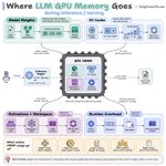
where does all the VRAM go during LLM inference?
(4 ways GPU memory is used)
loading the model is only the first part of the memory story.
once inference starts, GPU memory gets divided across multiple components, and some of them keep growing as context length, batch size, and concurrency increase.
the graphic breaks it into four useful buckets:
→ model weights are the mostly fixed part. once the model is loaded, their memory footprint stays roughly constant. the biggest lever here is precision. moving from FP16/BF16 to INT8 or INT4 reduces the number of bytes needed to store each parameter.
→ KV cache grows as generation continues. for every previous token, the model stores key and value tensors so attention can reuse them instead of recomputing the entire sequence. longer contexts mean a larger KV cache, and more concurrent requests mean more active caches sitting in memory.
→ activations and workspace hold temporary intermediate values needed while running attention, MLP layers, kernels, and other computations. this memory is reused across inference steps, but its size can still change with sequence length, batch size, and the kernels being executed.
→ runtime overhead comes from everything around the model itself. CUDA kernels, memory allocators, metadata, serving-engine buffers, and other runtime structures all consume some VRAM. it is usually smaller than the other buckets, but it is never zero.
this is why “the model fits on the GPU” and “the workload fits on the GPU” are two different statements.
a model may load comfortably, then run out of memory when you increase the context window, serve more users simultaneously, or increase the batch size.
it also explains why quantization can help beyond simply fitting a larger model. shrinking the weight footprint creates room that can instead be used for larger KV caches, more concurrent requests, or bigger batches.
that is the broader GPU lesson too.
performance is not just about how much arithmetic a GPU can do. it is also about what data occupies memory, how much of it moves during inference, and how often that data can be reused.
we wrote the full breakdown of how GPUs actually work and why memory movement sits at the center of LLM inference performance.
the article is quoted below.
Daily Dose of Data Science retweeted
Grok Bot masterclass.
In this video, I cover everything you need to understand and use Grok @Bot. Computer use, connectors, skills you teach with a screen recording, routines, and going from 1 to 14 bots that run like a company while I only talk to 4 of them.
Enjoy!
Chapters:
00:00 - Intro
01:22 - What a Grok Bot really is (a new hire with a laptop)
02:23 - Every bot gets its own computer
03:35 - Installation and pricing
05:01 - Creating your first bot (no system prompt to write)
06:29 - Routines: tasks your bot runs on a schedule
07:30 - Computer use and connected apps
11:50 - Skills: a recipe card for your AI
13:07 - Teach a Task: turning a screen recording into a skill
18:38 - One fat bot vs. 14 bots (and why both fail)
19:39 - Run it like a company: you, executives, workers
21:00 - The Notion task board that tracks every bot
21:31 - Designing the org with Claude
23:11 - Why my bots are named after TV characters
23:50 - Leadership in one group chat
26:31 - Chief of staff: inbox sweep across Gmail, Slack and X
27:10 - Head of content: post analysis and competitor watch
29:44 - Design team: on-brand illustrations and Typefully drafts
32:46 - Engineering team: GitHub issue to PR with one label
35:17 - Claude Code on your bot's computer
37:05 - Recap
38:12 - Outro
Cheers! :)

NVIDIA and Stanford challenged Jev.
(their new System 1 architecture runs up to 9x faster.)
It is called a Contrastive Language Model, or CLM.
Like Jev, CLM is not designed to generate text. It handles the small, repeated decisions inside AI systems, such as choosing a tool, ranking a patch, routing a request, or selecting the next action.
But CLM reaches those decisions differently.
Instead of generating an answer token by token, it treats decision-making as a retrieval problem.
Here is how it works.
1) Encode the state
CLM takes the current situation, such as an agent’s context or the state of a game, and converts it into a vector.
It uses a frozen Qwen3-8B model with a small trainable state projection head.
2) Encode every possible action
A separate action head converts each candidate into the same vector space.
In the Mario example, the candidates are left, jump, and right run. CLM does not invent a fourth option. It only evaluates the actions supplied by the application.
3) Learn which states and actions belong together
During training, the correct state-action pair is pulled closer while incorrect pairs are pushed apart.
A batch of B examples produces a B × B similarity matrix. The matching pairs sit on the diagonal. Every other pairing becomes a negative example.
This contrastive training uses InfoNCE, the same general mechanism behind systems such as CLIP and dense retrieval.
4) Turn similarity into a decision
At inference, CLM measures the cosine similarity between the state and every candidate action.
A softmax converts those scores into a probability distribution. The application can choose the winner, apply a confidence threshold, or escalate an uncertain result.
The real speed advantage comes from separating states and actions.
Actions can be embedded once and cached. If an agent repeatedly chooses between the same tools, CLM only needs to encode the changing state and compare it with stored action vectors.
That replaces repeated generation with one embedding pass and a set of cheap dot products.
The researchers report that CLM-8B matches Jev across computer-use, gaming, and tool-calling evaluations while reaching up to 9x lower latency. The improvement is largest when actions repeat or the candidate set grows.
CLM still has limits. It cannot generate new actions, its probabilities are relative to the supplied candidates, and its strongest verifier results require task-specific fine-tuning.
But its central idea is powerful.
The entire research is open-source, including the code.
Read more here: contrastive-lm.notion.site/
When software already knows the possible answers, an AI model should score them instead of generating more words.
We also wrote a full breakdown on how system one models like Jev work.
The article is quoted below.
Daily Dose of Data Science retweeted
Harness Engineering 2.0 is here!
We benchmark models all the time but the harness running the model can dramatically improve the result, cost, and execution time too.
And finally, devs just open-sourced Harness Arena, where you can test the same task across multiple harness and model combinations side by side.
You provide one task and then run it across several model x harness configs that you want to test.
Every config receives the same prompt, files, tools, skills, and evaluation checks. Harness Arena then returns:
- total cost
- execution time
- whether the task passed
- files and artifacts produced
If you want to try it yourself, it is implemented within the open-source HarnessRouter project.
Here's the repo: github.com/HarnessRouter/har…
(don't forget to star it ⭐ )
HarnessRouter is a plug-and-play infrastructure layer that lets you run any harness under a single interface, like:
- Codex
- Hermes
- Claude code
- DeepSeek Harness
- System One, powered by Jev
- And 25 more agent harnesses
In Harness Arena, the cheapest run does not automatically win.
A config must complete the task correctly first. Cost and execution time are compared only among the configurations that pass.
Here's the result from one Harness Arena test:
- Hermes + GPT-5.2: 5/5 successful runs using 0.47 credits
- Claude Code + Opus 4.8: 3/5 successful runs using 223 credits
That is around 474x difference in credits, while the more expensive configuration also failed two runs.
You can keep the model fixed to measure how much the harness changes the result. Or vary both to find the best harness and model pairing for that task.
This helps answer practical questions such as:
- Should this task run on Codex or Claude?
- Can a cheaper config still pass every check?
- Which setup is best to handle this workload?
Once you find the best config, you can run future tasks through it using the same Unified Harness Protocol (UHP) interface for sessions, streaming, files, artifacts, cancellation, and failures.
So you are no longer choosing an agent stack based only on a model leaderboard.
Instead, you can benchmark the complete runtime on the task your product actually needs to solve.
To dive deeper, my co-founder wrote an article explaining why model routing is different from harness routing, how UHP works, and what supporting multiple agent runtimes involves.
It also covers the local setup, a working request, and how sessions and files move through the system.
Read it below.
Daily Dose of Data Science retweeted
Harness Engineering 2.0 is here!
After protocols for tools, agent communication, and agent interfaces, harnesses now have one too.
Developers just built UHP (Unified Harness Protocol), a standardized interface for running agent tasks across any agent harness.
HarnessRouter is its open-source server implementation.
Here’s how it works:
- The product backend sends a task with a `harness_id`.
- HarnessRouter starts the selected harness in its own session.
- The harness runs its native agent loop and streams back progress.
- Files, artifacts, failures, and the final output return through the same interface.
Without UHP, integrating every harness needs separate handling for task execution, sessions, streaming, files, recovery, and output formats.
With UHP, Codex, Claude Code, Gemini CLI, Hermes, Pi, and other harnesses can plug into the same product backend while keeping their native tools, skills, models, and agent loops.
This means developers can:
- Switch harnesses without rebuilding the product integration.
- Run the same task across different harnesses.
- Add new harnesses without maintaining another execution stack.
HarnessRouter currently supports 30 harness bases.
Here’s the repo: github.com/HarnessRouter/har…
(don’t forget to star it ⭐)
As per official benchmarks, changing only the harness while keeping the model fixed reduced costs by 25% to 64% across several healthcare compliance tasks.
And changing both the harness and model widened the difference to 99.8% between the highest and lowest-cost configurations.
Developers can test their own workloads across different configurations using Harness Arena.
Alibaba Cloud's Qoder has also adopted UHP, making it available as an agent backend through the HarnessRouter API.
If you want to dive deeper, I already wrote an article that explains why model routing is different from harness routing and what supporting multiple agent runtimes actually involves.
It also covers UHP, the local setup, a working API call, and how sessions and files work.
Read it below.
Daily Dose of Data Science retweeted
A new technique just made attention 23x faster!
At 10M tokens, sparse attention slows down not because of attention itself but rather because of deciding which keys to attend to.
Let's understand why and how a new technique solves it without scanning every key.
1) Full attention at long context:
In full attention, every query is compared against every earlier key. This leads to O(T^2) complexity for prefill, and at 10M tokens it dominates the forward pass.
2) Sparse attention:
Sparse attention lets each query read only a small set of <k> keys instead of all of them, so the attention becomes cheap.
But something still has to pick those <k> keys, and at long context, this step becomes the bottleneck.
3) Why picking keys is still quadratic:
DeepSeek's DSA uses a lightning indexer that scores every earlier key. GLM-5.3-Flash pools 4 keys into 1 before scoring. NSA, MoBA, and Quest score blocks of nearby keys.
Each of them scans the whole context for every query, so the indexer stays O(T^2), and at 10M tokens, it takes 98% of the layer's time.
Block methods have another issue. Blocks group keys by position, so one relevant key within filler can get averaged away in the block summary.
4) How LSA picks keys:
Latent Sparse Attention (LSA) is a new approach that groups keys by meaning instead of position.
- Each key is projected into a 64-dim index space, and every 4 consecutive keys are pooled into one.
- When a 512-key block fills up, it's clustered into buckets of ~8 similar keys, with one centroid per bucket. Finished blocks are never rebuilt.
- A query scores only the centroids, keeps the top 1,024 buckets, and expands them into 4,096 keys, plus 4 sink tokens and the 512 most recent keys.
- Exact FlashAttention then runs over that list with an unchanged kernel.
If you've built RAG, this is like cluster-based vector search running inside attention. The kernel design even cites FAISS.
At 10M tokens, LSA's prefill is 72.4x faster than full attention on Qwen-3.8-27B and 22.7x faster than GLM-5.3-Flash's own sparse attention.
The time to first token improves:
- 9.2x on Qwen
- 2.2x on GLM
Below ~512k tokens, it's roughly break-even.
Here's the paper: arxiv.org/abs/2610.42147
That said, LSA attempts to find the keys more cheaply, not storing them. The KV cache still grows linearly with context, and at 10M tokens, managing that memory becomes the next engineering problem.
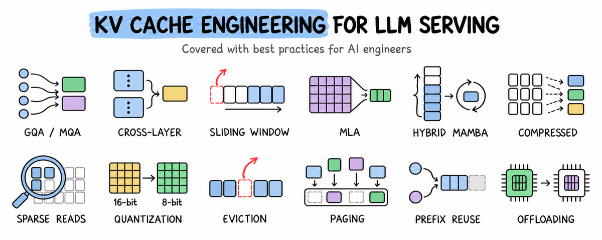
I wrote an article on how 12 ways serving systems handle it, covering paging, offloading, quantizing, and more.
Read it below.