Physical Review X

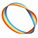
ALT A rainbow band depicted as a vortex loop, where the band appears to be twisting and folding over itself in places. The loop is a ribbon, and each linking of the ribbon contains a different phase.

ALT A figure illustrating the paper’s central result: a new Spectral Small-Incremental-Entangling theorem puts a universal limit on how quickly the detailed structure of quantum entanglement can change. At left, two colored spheres labeled A and B represent two interacting quantum subsystems, connected by an interaction. At right, a plot shows the time-evolving entanglement spectrum, with squared Schmidt coefficients decreasing with coefficient index and following a 1/s2 tail.

ALT A figure compares the dissociation energy results of this work to previous reported measurements. The top third of the plot is shaded pink, and labeled para-H2. The bottom section, labeled ortho-H2, is shaded blue. In the plot, points with error bars are stacked vertically and labeled with the corresponding paper they are from. From top to bottom, those labels read: This work, Beyer et al. 2019a, This Work, Holsch et al. 2019b, Cheng et al. 2018c, Altmann et al. 2018d, and Liu et al. 2009e.

ALT Two diagrams show a multicomponent mixture with a blue background representing the solvent. The diagram labeled “Homogeneous” is a schematic of a homogeneous state. The solutes are depicted by around 30 differently colored circles randomly and roughly evenly distributed around the box. The diagram labeled “Phase separated” is a schematic of a phase separated state, where several droplets of diverse sizes and compositions can coexist. In three regions, the multicolored circles are randomly distributed or clustered to represent three droplets, one small (top right), one medium (top left) and one large (bottom).

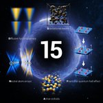
ALT Against a dark, star-filled space background, a glowing blue ring surrounds a large white "15" at the center, marking the journal's 15th anniversary. Five illustrated research topics are arranged around the ring: a colorful visualization labeled "Diffusive hydrodynamics" at upper left; a 3D lattice of black spheres labeled "Gravitational waves" at upper center; layered blue panels with red particles and upward arrows labeled "Fractional quantum hall effect" at right; intersecting blue and gold light beams labeled "Neutral atom arrays" at lower left; and a cluster of blue and gold spheres labeled "Active colloids" at bottom center.

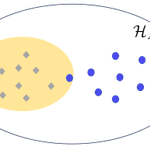
ALT A diagram depicting the concept of localizable quantumness. A white oval, labeled HA, contains a smaller yellow oval, representing the free projected state set, with eight gray diamonds scattered randomly. Seven blue dots sit within the larger white oval, all outside the yellow oval except one. If the target state exhibits localizable quantumness, then its projected ensemble, shown by the blue dots, differs significantly from the projected ensemble of any free state ρ, shown by the grey diamonds. This difference can be utilized to certify the quantumness of the target state by examining the small subsystem A.

ALT Schematic of an antiphase boundary in an antiferromagnetic topological insulator. Two cuboids sit next to each other. The left is pink with a blue horizontal layer through its middle, the right is blue with a pink layer through its middle. Both have thin red arrows located at the domain boundaries running counter-clockwise on the left cuboid’s top surface and clockwise on the right one, representing the chiral edge current. Short thick red arrows point out of the surface of the left cuboid, positive z-direction, denoting the magnetic moments pointing upward. On the right, short blue arrows denote the magnetic moments point down. Above the cuboids are curved black lines schematically showing the surface band structures and surface Brillouin zone for respective domains and their boundaries. A + on the left and a − on the right indicate the signs of the Chern number.

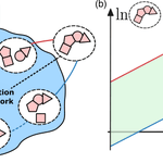
ALT A two-panel diagram illustrating how energy constrains a chemical reaction network. At left, clusters of pink shapes represent chemical species connected by reaction pathways within a blue network supplied with fuel by a chemical reservoir. Red and blue paths highlight those that set the thermodynamic limits. At right, a graph with logarithmic concentration axes shows a green band between a red upper bound and a blue lower bound. This bound is the thermodynamic space containing the possible steady-state concentrations. Its width increases with the nonequilibrium driving force, showing how a larger energy budget expands the network’s operating range.

ALT An abstract depiction of gravitational waves, shown as black ripples in the background with two intersecting beams in the foreground. Above is a pastel-colored cloud filled with spheres and squiggly lines.

ALT Rectangle diagram titled “All 3D topological phases in K-theory.” A large yellow rectangle represents 2D topological invariants and is divided into three columns: Gapless, TI/TSC, and Atomic states. Inside it is a smaller orange rectangle (1D invariants), with a red-and-orange striped region within labeled "Symmetry indicators.” A small green rectangle (3D invariants) sits on top of the TI/TSC column. A legend on the right identifies each color: red for 0D, orange for 1D, yellow for 2D, and green for 3D invariants.

ALT A two-panel diagram comparing conventional and quantum-enhanced sensing of classical fields. In the top panel, conventional sensing measures a complex field along selected axes, producing separate projections that lose information, or a blurred distribution due to added vacuum noise. In the bottom panel, quantum-enhanced Bell Quantum Signal Learning uses entangled two-mode squeezed states, with one mode probing the field and the other stored as a reference. Beam splitters and homodyne measurements combine the modes to recover multiple properties of the field with greater precision and without choosing a single measurement direction in advance.

ALT Top row: two scanning electron microscope images on a dark blue-green background, each with a white "1 µm" scale bar. Left image labeled "Rough" shows an electrode tip with a jagged edge. Right image labeled "Sharp" shows an electrode tip with a smooth edge. Bottom row: two line graphs plotting conductance G(S) against voltage (mV, from -10 to 10) both labeled "FeTe0.55Se0.4 ." Left graph, labeled “Rough," RN = 106 Ω, shows a red line with a single sharp peak centered at zero voltage. Right graph, labeled "Sharp," RN = 276 Ω, shows a blue line forming a flat-topped plateau between about -2 and 2 mV.

ALT A schematic showing two sets of arrows extending from a central point in 3D space. Black axes extend from the center, and a light gray grid forms a background. Orange arrows on the left are labeled “Tr ρ = 1,” while blue arrows on the right are labeled “Tr ρ = 0.” Each set follows a red triangular path marked with time-evolution expressions. At the bottom in the gridded space are labels “𝒦₀” in orange and “𝒦α” in blue.

ALT Panel (a) consists of a graph plotting the dynamics of kurtosis of rapidity distribution as a function of rescaled time on the x-axis. The graph contains six lines corresponding to V0 = 1 (dark blue), V0 = 2 (medium blue), V0 = 3 (light blue), V0 = 4 (light green), V0 = 5 (medium green), and V0 = 6 (dark green). Panel (b) plots the evolutions of distributions of rapidity on the y-axis, rescaled time on the y-axis, and 𝛳 on the z-axis. HR for V0 = 4 is plotted with a light blue line, and gBBGKY for V0 = 4 is plotted with a dark blue line. Panels (c, e, f) present similar graphs plotting the evolution two-point correlation function. Panel (d) presents a similar graph as panel (a), plotting the dynamics of the kinetic energy function. In all the graphs, dots represent the molecular dynamics of the system while solid lines represent the prediction by gBBGKY.

ALT Six-panel figure on black, arranged in two rows of three. Each panel except top-right shows a purple-to-yellow heatmap with a white parallelogram outline marking the moiré unit cell and a green dot marking a fixed hole position. Some show a single bright glowing blob, others show three bright spots at the parallelogram's corners, and one shows a glow at the center and corner. The top-right panel is a separate schematic with red and blue circles showing electron and hole doping with curved arrows.

ALT A phase map of shock-compressed MgO showing temperature versus pressure for three crystal orientations: [111] shown in red, [110] in blue, and [100] in green. The measurements follow different paths through the B1 and B2 solid phases before converging near complete melting at about 572 GPa and 13,200 K. X-ray diffraction ranges below the plot show orientation-dependent B1-to-B2 transition behavior. An inset compares MgO’s melt curve with those of Ta, Fe, SiO2, diamond, and MgSiO3, showing MgO’s unusually high melting temperature. A top axis relates pressure to estimated core-mantle boundary pressures in super-Earths.

ALT Two diagrams with x-y-z axes show topological charge polarization induced by an external magnetic field in a magnetic AXI, and topological nonlocal spin polarization induced by an external magnetic field in a T-DAXI. Both diagrams show a green cuboid, labeled either “AXI” or “T-DAXI,” with a red arrow labeled either “P” or “Ps,” representing the induced charge polarization, and an external magnetic field, B, both pointing upward. For AXI, positive-charge circles run along the bottom and negative-charge circles run along the top. For T-DAXI, left-pointing arrows, representing “spin sy down,” run along the bottom and right-pointing arrows, representing “spin sy up,” run along the top.

ALT A bell-shaped normal distribution shown in blue–symmetric and peaking at x = α. Below the curve is a series of five green circle clocks with one hand. From left to right, the hand rotates from roughly the 11 o’clock position counter clockwise to roughly 7 o’clock, with 9 o’clock sitting under the bell curve peak. The clocks represent the Bloch state projections of a qubit. The bell curve is a probability distribution of the oscillator position. The spread of ticks in the clock around the target state on the yz-plane of the Bloch sphere illustrates the over- and under-rotations arising from Gaussian position uncertainty.

ALT Diagram illustrating hematite's crystal and magnetic structure across a temperature scale from TM ≈ 255 K to TN ≈ 950 K. Three 3D rhombus-shaped structures are shown side by side, each containing orange spheres (Fe³⁺ ions) connected by gray spheres (O²⁻ ions). Red arrows show spin orientation. A legend identifies the orange and gray spheres. Below, two hexagonal top-down views show red arrows for L and black arrows for M pointing in different directions.